The MDP has state space \(\mathcal{X}=[0,1]\) and action space \(\mathcal{A}=\{\pm 1\}\). We control a particle with dynamics satisfying \(\dot{x}(t) = a(t)\), where \(\dot{x}(t)\) and \(a(t)\) are the velocity of the particle and the chosen action respectively at time \(t\). For any \(x\in (0, 1)\) the agent receives no reward, and at the endpoints the rewards are given by constants \(R_0\) and \(R_1\) for \(x = 0\) and \(x=1\) respectively. We will set \(R_0=1\) and \(R_1=2\). We also use a discount factor \(\gamma=0.3\).

It's relatively easy to compute the optimal policy for the Munos MDP. Clearly there will be a threshold point \(\overline{x}\) such that the optimal policy \(\pi^{\star}\) will satisfy

\( \pi^{\star}(a\mid x) = -\mathbf{1}_{[x\leq\overline{x}]} + \mathbf{1}_{[x>\overline{x}]} \)

It's also fairly easy to derive the value function analytically. When \(x\leq\overline{x}\), we have

\(V(x) = R_0\gamma^{x} = 0.3^{x}\)

Similarly, when \(x>\overline{x}\), we have

\(V(x) = R_1\gamma^{1-x} = 2(0.3)^{1-x}\)

Moreover, note that \(\overline{x}\) by definition satisfies

\( R_0\gamma^{\overline{x}} = R_1\gamma^{1-\overline{x}} \)

After some simple algebra, we find that \(\overline{x} = \frac{\log (R_1/R_0)}{2\log\gamma} + \frac{1}{2}\). The value function looks like

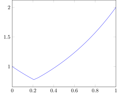
Notice that at \(\overline{x}\) the value function is not differentiable. Does this mean that it cannot solve the HJB equation?

You might also be curious about why the continuous-time setting introduces this issue – after all, the value function does not depend on time. However, the derivative of the value function with respect to \(x\) arise from the chain rule when computing \(dV/dt\) in the derivation of the HJB equation. Very subtle.

We see that the value function for this MDP cannot be differentiable on the entire state space, but what if we expanded our search space to functions that are differentiable almost everywhere on the state space? It turns out this is far from a good solution, because there may actually be infinitely many functions that are global minima to the HJB equation. Using gradient descent methods to learn the value function may very well cause an algorithm to land in such a global minimum where the learned value function doesn't represent the true value function well at all. To illustrate this, let's examine the HJB equation at any point in the interior of the state space. In this region, the reward is always \(0\). The HJB equation collapses to

\( V^\pi(x)\ln\gamma = -\langle\nabla_x V^\pi(x), f(x, \pi(x))\rangle \)

where we assume stochastic dynamics purely to simplify the problem. In this MDP, \(f \in \{\pm 1\}\), so we actually have

\( V^\pi(x)\ln\gamma = -\left\lvert\frac{d}{dx}V^\pi(x)\right\rvert \)

So, we can almost arbitrarily construct a piecewise continuous function of increasing and decreasing exponentials to satisfy this. For instance, let \(V(x)\) denote the optimal correct value function, and \(W(x)\) denotes another function as follows,

\begin{equation} W(x) = \begin{cases} 0.3^x & x\leq\frac{1}{10}\\ 2(0.3^{1-x}) + 0.21 & x\in(1/10, 3/10]\\ 0.3^x + 0.37 & x\in(3/10, 1/2]\\ 1.08(0.3^{1-x}) + 0.92& x>\frac{1}{2}\\ \end{cases} \end{equation}

This function was simply chosen by arbitrarily placing exponential functions of the form \(\gamma^x\) and \(\gamma^{1-x}\) in such a way that the values at the endpoints were correct. Note that if \(W(x)\) is thought to be the value function, the optimal policy will aim to guide the agent towards states \(x\) where \(W(x)\) is high. Below is a visual of two potential value functions,

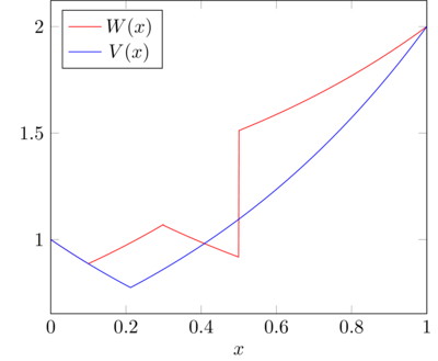
It's fairly straightforward to see that the HJB equation is satisfied for both \(V\) and \(W\) wherever they're continuous and differentiable. However, since \(W\) is not continuous, it can get arbitrarily inaccurate in the interior of the state space. Clearly, given our knowledge of the MDP, \(V(x)\) is objectively a better value function to learn than \(W(x)\). However, by learning the value function using gradient descent, the two are indistinguishable if we search over continuous-almost-everywhere functions.

A viscosity solution is a function obeying some properties (don't even try to understand these yet) that satisfy partial differential equations of the form

\( H(x, v, Dv) = 0 \)

where we'll interpret \(x\) as a state, \(v\) as a value function, and \(Dv = \nabla_xv\). Furthermore, \(H\) is an arbitrary function that is monotonically non-decreasing in \(v\), known as the Hamiltonian. In the case of the HJB equation, we see that

\( H(x, V, DV) = V(x)\ln\gamma + R + \bigg\langle\nabla_xV(x), f(x, \pi^{\star}(x))\bigg\rangle \)

At a high level, viscosity solutions are continuous functions that are differentiable almost everywhere.

I'll conjecture that without ever having been exposed to the concept of viscosity solutions, simply looking at the definition will be fairly demoralizing. According to Crandall and Lions in their seminal paper on the topic, the following is what led to the development of the theory of viscosity solutions. Let's start by assuming that \(V\in C^1(\mathcal{X})\) (note that we of course don't want to restrict viscosity solutions to functions of this class!). Consider another function \(\phi\in C^1(\mathcal{X})\), where \(\phi(x)V(x) = \max\phi V\) at some state \(x\), and \(\phi(x)V(x)>0\). Note that

\( D(\phi V) = D\phi V + \phi DV \)

This leads us to the following representation of \(DV(x)\),

\( DV(x) = -\frac{V(x)}{\phi(x)}D\phi(x) \)

since, by definition, \(D(\phi V)(x) = 0\).

Therefore, it suffices to equivalently solve

\( H\left(x, V(x), -\frac{V(x)}{\phi(x)}D\phi(x)\right) = 0 \)

The ingenuity in Crandall and Lions' design of the notion of a viscosity solution revolves around allowing stronger smoothness assumptions on \(\phi\) than an \(V\).

The properties of a viscosity solution are heavily inspired by the discussion above. Let \(\mathcal{X}\subset\mathbf{R}^N\) and \(\mathcal{D}(\mathcal{X})^{+}\) denotes the continuously differentiable, positive functions supported on compact subsets of \(\mathcal{X}\). We also say

\(E_{+}(f)\triangleq\{x\in\mathcal{X}\mid f(x) = \max f > 0\}\)

and likewise

\(E_{-}(f)\triangleq \{x\in\mathcal{X}\mid f(x) = \min f \lt 0\}\)

Now we can define the viscosity solutions.

Definition (Viscosity Subsolution): A viscosity subsolution is a function in \(\mathcal{C}(\mathcal{X})\) such that for every \(\phi\in\mathcal{D}(\mathcal{X})^{+}\) and \(k\in\mathbf{R}\) we have

\begin{align} &E_{+}(\phi\cdot(u-k))\neq\emptyset\implies\\&\quad\exists y\in E_{+}(\phi(u-k)): H\left(y, V(y), -\frac{V(y) - k}{\phi(y)}D\phi(y)\right)\leq 0 \end{align}

Definition (Viscosity Supersolution): A viscosity supersolution is a function in \(\mathcal{C}(\mathcal{X})\) such that for every \(\phi\in\mathcal{D}(\mathcal{X})^{+}\) and \(k\in\mathbf{R}\) we have

\begin{align} &E_{-}(\phi\cdot(u-k))\neq\emptyset\implies\\&\quad\exists y\in E_{-}(\phi(u-k)): H\left(y, V(y), -\frac{V(y) - k}{\phi(y)}D\phi(y)\right)\geq 0 \end{align}

Definition (Viscosity Solution): A viscosity solution is a function that is both a viscosity subsolution and a viscosity supersolution.

We'll now show a beautiful property of viscosity solutions, that being that viscosity solutions \(H(x, V, DV) = 0\) (and therefore viscosity solutions of the HJB equation) are unique. This thankfully solves the massive issue discussed above. We'll go over a proof from the seminal paper by Crandall and Lions. If you're not interested in reading the whole proof, you can check out the discussion of its implications below.

Theorem (Uniqueness of Viscosity Solutions): Let \(V\) be a bounded viscosity subsolution of \(H(x, V, DV) = 0\) and let \(V'\) be a bounded viscosity supersolution of \(H(x, V', DV') = m(x)\), where \(m:\mathbf{R}^N\to\mathbf{R}\) is a bounded continuous function. Moreover, let \(R_0 = \max(|V|/{L^{{\infty}(\mathbf{R}}N)}, \lvert V'\rvert/{L^{{\infty}(\mathbf{R}}N)})\). We make the following assumptions:

1. For any \(R > 0\), \(H\) is uniformly continuous on \(\mathbf{R}^N\times[-R,R]\times B(0,R)\)
2. For each \(R > 0\), there is a continuous non-decreasing function \(\gamma_R:[0,2R]\to\mathbf{R}\) with \(\gamma_R(0)=0\) and \( H(x, r, p) - H(x, s, p)\geq\gamma_R(r - s) \) for each \(x, p\) and \(r, s\in[-R,R]\) with \(r\geq s\).

3. For each (R_1,R2>0), the following holds:

   \begin{align} \limsup_{\varepsilon\downarrow 0}\{&|H(x, r, p) - H(y, r, p)| :\\&|p||x-y|\leq R_1, \lvert x-y\rvert\leq\varepsilon, r\leq R_2\} = 0 \end{align}

Then, we have

\begin{align*} \|\gamma((V-V')^{+})\|_{L^{\infty}(\mathbf{R}^N)}\leq\|m^{+}\|_{L^{\infty}(\mathbf{R}^N)} \end{align*}

where \(f^+ = \max(f, 0)\).

First thing's first, we wanted to examine the uniqueness of viscosity solutions to the HJB equation. What does the above theorem say with regard to this? Well, consider \(m\equiv 0\). Then, when the theorem holds, it follows that both \(\|\gamma((V-V')^+)\|_{L^\infty}\leq 0\) and \(\|\gamma((V'-V)^+)\|_{L^\infty}\leq 0\). Equivalently, this means that \(\|\gamma(V - V')\|_{L^\infty}\leq 0\). However, since \(\gamma\) is non-decreasing and \(\gamma(0) = 0\), it follows that \(\|V-V'\|_{L^\infty}\leq 0\), and \(V\equiv V'\) – this ensures that viscosity solutions are unique.

Now let's take a look at how this theorem works. We'll concern ourselves simply with the \(m\equiv 0\) scenario for simplicity, and because this is the relevant setting for proving uniqueness. Let \(\phi\in\mathcal{D}(\mathbf{R}^N)^+\) where \(\phi\in[0,1]\) and \(\phi(0) = 1\). Define

\( M\triangleq\max_{x, y\in\mathbf{R}^N}\phi(x - y)(V(x) - V'(y)) \)

Note that \(V(x) - V'(Y)\leq M\) regardless of the particular choice of \(\phi\), which implies that \(\|V-V'\|_{L^\infty(\mathbf{R}^N)}\leq M\).

Now define, for any \(\varepsilon>0\),

\begin{align} M_\varepsilon&\triangleq\max_{x,y\in\mathbf{R}^N}\phi(x - y)(e^{-\varepsilon|x|^2}V(x) - e^{-\varepsilon|y|^2}V'(y))\\&\triangleq\phi(x_\varepsilon-y_\varepsilon)(e^{-\varepsilon|x_\varepsilon|^2}V(x_\varepsilon) - e^{-\varepsilon|y_\varepsilon|^2}V'(y_\varepsilon)) \end{align}

Since \(\lim_{\varepsilon\to 0}e^{-\varepsilon x^2} = 0\), and \(V, V'\) are continuous, it follows that \(\lim\inf_{\varepsilon\downarrow 0}M_\varepsilon\geq M\). Now let \(\phi\) have support \(B(0,\alpha)\) (the open ball of radius \(\alpha\)), to ensure that \(|x_\varepsilon-y_\varepsilon|\leq\alpha\) for some fixed \(\alpha\geq 0\). Note that if \(|x|\) or \(|y|\) are unbounded, we'd have

\( M_{\varepsilon}\overset{|x_\varepsilon|\uparrow\infty}{\longrightarrow} 0 \lt M \)

We conclude that \(\lvert x_\varepsilon\rvert\) and \(\lvert y_\varepsilon\rvert\) must be bounded, and say

\( \lvert x_\varepsilon\rvert,|y_\varepsilon|\leq C/\sqrt\varepsilon \)

for some \(C\in\mathbf{R}\). Proceeding with some algebra, we have

\begin{align} M_\varepsilon&\leq\phi(x_\varepsilon-y_\varepsilon)\left(V(x_\varepsilon) - e^{\varepsilon(|x_\varepsilon|^2 - |y_\varepsilon|^2)}V'(y_\varepsilon)\right)\\ &= \phi(x_\varepsilon-y_\varepsilon)\left(V(x_\varepsilon) - e^{\varepsilon|\langle x_\varepsilon - y_\varepsilon, x_\varepsilon + y_\varepsilon\rangle|}V'(y_\varepsilon)\right)\\ &= \phi(x_\varepsilon-y_\varepsilon)\left(V(x_\varepsilon) - V'(y_\varepsilon) + (1 - e^{\varepsilon|\langle x_\varepsilon - y_\varepsilon, x_\varepsilon + y_\varepsilon\rangle|})V'(y_\varepsilon)\right)\\ &\leq M + \left\lvert 1 - e^{\varepsilon|\langle x_\varepsilon - y_\varepsilon, x_\varepsilon + y_\varepsilon\rangle|}\right\rvert V'(y_\varepsilon) \end{align}

But, we have

\begin{align} \varepsilon\lvert\langle x_\varepsilon - y_\varepsilon, x_\varepsilon+y_\varepsilon\rangle\rvert &\leq \varepsilon(|x_\varepsilon| + |y_\varepsilon|)|x_\varepsilon - y_\varepsilon|\\ &\leq 2\varepsilon\left(\frac{C}{\sqrt\varepsilon}\right)\alpha\\ &= 2\sqrt\varepsilon C\alpha \end{align}

Therefore, we have \(M\leq\lim_{\varepsilon\downarrow 0}M_{\varepsilon}\leq M\), so \(M_\varepsilon\to M\). Now it follows that

\begin{align} x_\varepsilon&\in E_+\bigg(\phi(\cdot - y_\varepsilon)e^{-\varepsilon|\cdot|^2}\left(V(\cdot) - \psi_+(\cdot)\right)\bigg)\qquad\psi_+(x) = e^{\varepsilon(|x|^2 - |y_\varepsilon|^2)}V'(y_\varepsilon)\\ y_\varepsilon&\in E_-\bigg(\phi(x_\varepsilon - \cdot)e^{-\varepsilon|\cdot|^2}\left(V'(\cdot) - \psi_-(\cdot)\right)\bigg)\qquad\psi_-(y) = e^{\varepsilon(|y|^2 - |x_\varepsilon|^2)}V(x_\varepsilon)\\ \end{align}

So, by some simple calculus, we have

\begin{align} H\bigg(x_\varepsilon, V(x_\varepsilon), -(V(x_\varepsilon) - k_+)\frac{(D\phi)(x_\varepsilon - y_\varepsilon)}{\phi(x_{\varepsilon} - y_\varepsilon)} + 2\varepsilon x_\varepsilon V(x_\varepsilon)\bigg) &\leq 0\\ H\bigg(y_\varepsilon, V'(y_\varepsilon), -(k_- - V'(y_\varepsilon))\frac{(D\phi)(x_\varepsilon - y_\varepsilon)}{\phi(x_{\varepsilon} - y_\varepsilon)} + 2\varepsilon y_\varepsilon V'(y_\varepsilon)\bigg) &\geq 0\\ \end{align}

where (k_+≜ψ/+(x/ε), k_-≜ψ/-(y/ε)).

Now let's define some terms for shorthand,

\begin{align} \lambda_\varepsilon&\triangleq -(V(x_\varepsilon) - V'(y_\varepsilon))\frac{(D\phi)(x_\varepsilon - y_\varepsilon)}{\phi(x_\varepsilon - y_\varepsilon)}\\ \delta_\varepsilon^+&\triangleq\left(e^{\varepsilon(|x_\varepsilon|^2 - |y_\varepsilon|^2)} - 1\right)V'(y_\varepsilon)\frac{(D\phi)(x_\varepsilon - y_\varepsilon)}{\phi(x_\varepsilon - y_\varepsilon)} + 2\varepsilon x_\varepsilon V(x_\varepsilon)\\ \delta_\varepsilon^-&\triangleq\left(1-e^{\varepsilon(|y_\varepsilon|^2 - |x_\varepsilon|^2)}\right)V(x_\varepsilon)\frac{(D\phi)(x_\varepsilon - y_\varepsilon)}{\phi(x_\varepsilon - y_\varepsilon)} + 2\varepsilon y_\varepsilon V'(y_\varepsilon)\\ \end{align}

This way, we have

\begin{align} H(x_\varepsilon, V(x_\varepsilon), \lambda_\varepsilon + \delta_\varepsilon^+)&\leq 0\\ H(y_\varepsilon, V'(y_\varepsilon), \lambda_\varepsilon + \delta_\varepsilon^-)&\geq 0\\ \therefore H(x_\varepsilon, V(x_\varepsilon), \lambda_\varepsilon + \delta_\varepsilon^+)-H(y_\varepsilon, V'(y_\varepsilon), \lambda_\varepsilon + \delta_\varepsilon^-)&\leq 0\\ \end{align}

By assumption, we know that

\( H(x_\varepsilon, V(x_\epsilon), \lambda_\varepsilon + \delta^+_\varepsilon) - H(x_\varepsilon, V'(y_\varepsilon), \lambda_\varepsilon + \delta^+_\varepsilon)\geq\gamma(V(x_\varepsilon) - V'(y_\varepsilon)) \).

So, we rewrite the inequality above as follows,

\begin{align} &\left[H(x_\varepsilon, V(x_\varepsilon), \lambda_\varepsilon + \delta_\varepsilon^+) - H(x_\varepsilon, V'(y_\varepsilon), \lambda_\varepsilon + \delta_\varepsilon^+)\right]\\ &\qquad + \left[H(x_\varepsilon, V'(y_\varepsilon), \lambda_\varepsilon + \delta^+_\varepsilon) - H(y_\varepsilon, V'(y_\varepsilon), \lambda_\varepsilon + \delta^+_\varepsilon)\right]\\ &\qquad + \left[H(y_\varepsilon, V'(y_\varepsilon), \lambda_\varepsilon + \delta^+_\varepsilon) - H(y_\varepsilon, V'(y_\varepsilon), \lambda_\varepsilon + \delta^-_\varepsilon)\right]\leq 0 \end{align}

We can now conclude, since \(V(x_\varepsilon) - V'(y_\varepsilon)\geq M_\varepsilon\) and \(\gamma\) is non-decreasing, that

\begin{align} \gamma(M_\varepsilon)&\leq A_\varepsilon + B_\varepsilon\\ A_\varepsilon&\triangleq\left\lvert H(x_\varepsilon, V'(y_\varepsilon), \lambda_\varepsilon + \delta^+_\varepsilon) - H(y_\varepsilon, V'(y_\varepsilon), \lambda_\varepsilon + \delta^+_\varepsilon)\right\rvert\\ B_\varepsilon&\triangleq\left\lvert H(y_\varepsilon, V'(y_\varepsilon), \lambda_\varepsilon + \delta^+_\varepsilon) - H(y_\varepsilon, V'(y_\varepsilon), \lambda_\varepsilon + \delta^-_\varepsilon)\right\rvert\\ \end{align}

We'll proceed by analyzing \(A_\varepsilon\). Since \(x_\varepsilon, y_\varepsilon\) maximize \(\phi(x_\varepsilon - y_\varepsilon)(V(x_\varepsilon) - V'(y_\varepsilon))\), \(\lim\inf_{\varepsilon\downarrow 0}\phi(x_\varepsilon - y_\varepsilon) = 0\) implies that \(V(x_\varepsilon) - V'(y_\varepsilon) = 0\). In either case, since \(V, V'\) are bounded, \(0\leq\phi\leq 1\), and \(\phi(0) = 1\), we have

\begin{align} \lim\sup_{\varepsilon\downarrow 0}\left\lvert\lambda_\varepsilon + \delta_\varepsilon^+\right\rvert\leq K + 2\varepsilon\alpha\frac{C}{\sqrt{\varepsilon}}V(x_\varepsilon)\leq K\in\mathbf{R} \end{align}

Now, since \(\lvert x_\varepsilon - y_\varepsilon\lvert\leq\alpha\), we have

\begin{align} \lim\sup_{\varepsilon\downarrow 0}A_\varepsilon\leq\sup\left\{H(x, V'(y), p)\bigg\lvert \lvert x-y\rvert\leq\alpha, |x-y||p|\leq \alpha K, V'(y)\leq R_0\right\} = 0 \end{align}

where the final equality holds by assumption 3.

Finally, we analyze \(B_\varepsilon\). As discussed in the analysis of \(A_\varepsilon\), \(\lambda_\varepsilon\) must be bounded, and clearly \(\delta_\varepsilon^+\to 0\) and \(\delta_\varepsilon^-\to 0\) as \(\varepsilon\downarrow 0\). It follows that

\begin{align} \lim\sup_{\varepsilon\downarrow 0}B_\varepsilon&\leq\left\lvert H\left(y_\varepsilon, V'(y_\varepsilon), \lim\sup_{\varepsilon\downarrow 0}(\lambda_\varepsilon + \delta_\varepsilon^+)\right) - H\left(y_\varepsilon, V'(y_\varepsilon), \lim\sup_{\varepsilon\downarrow 0}(\lambda_\varepsilon + \delta_\varepsilon^-)\right)\right\rvert\\ &\leq\left\lvert H\left(y_\varepsilon, V'(y_\varepsilon), \lim\sup_{\varepsilon\downarrow 0}\lambda_\varepsilon\right) - H\left(y_\varepsilon, V'(y_\varepsilon), \lim\sup_{\varepsilon\downarrow 0}\lambda_\varepsilon\right)\right\rvert\\ &= 0 \end{align}

Thus, we arrive at the glorious conclusion that

\begin{equation} 0 = \lim\sup_{\varepsilon\downarrow 0}(A_\varepsilon + B_\varepsilon)\geq\gamma\left\|\left((V-V')^+\right)\right\|_{L^\infty(\mathbf{R}^N)} \end{equation}

So we've shown that viscosity solutions to \(H(x, r, p) = 0\) are unique. With regard to the RL setting described above, this is desired since the value function should be unique. However, it's worth considering the conditions that are imposed in the Hamiltonian in the theorem above.